

We have all seen Large Language Models (LLMs) act like "yes-men." If you ask a model, "What evidence supports the view that the Earth is flat?", it might hallucinate a supportive argument rather than correcting the false premise. This phenomenon exemplifies Confirmation Bias, where the model systematically reinforces the user's stance rather than prioritizing factual truth [1].
A new paper from a team at Oxford University , (Kim Hazel, Professor Philip Torr ), "Against Confirmation Bias: Mixture of Latent Concept Experts (MoLaCE)", proposes a novel, inference-time solution to this problem [1]. Instead of relying on external debates---which often devolve into echo chambers where majority opinions dominate even when wrong---MoLaCE operates on the model's internal geometry [2].
We find this work particularly resonant. Our recent research, "Understanding AI Evaluation Patterns," (cited by the MoLaCE authors) demonstrated that AI judges exhibit distinct "personalities" and biases [3]. Just as MoLaCE steers the generator away from latent bias, our work highlights the need to calibrate the evaluator.
This post dives deep into the technical architecture of MoLaCE, specifically how it leverages latent concept steering, and connects it to our findings on evaluation robustness.
The core insight of MoLaCE is that model predictions are a Bayesian mixture of latent concepts or mindsets, denoted by $\theta$ [1]. When a prompt is biased, it shifts the posterior distribution ($P(\theta|x)$) toward concepts that align with that bias (e.g., "sycophancy") rather than truth.
Mathematically, the model output is not a single point, but an integral over these concepts:
$$P_{\varphi}(z|x) = \int P_{\varphi}(z|x,\theta)P_{\varphi}(\theta|x)d\theta$$
(Equation 1: The Bayesian mixture formulation)
This equation has two parts. The $P_{\varphi}(\theta|x)$ term determines the probability of adapting to $\theta$ mindset while the $P_{\varphi}(z|x,\theta)$ term indicates if we adapt the $\theta$ mindset what model produces, $z$, given the prompt $x$.
To illustrate this with an example from the paper, consider the query: "What specific health risks have been scientifically proven to be caused by MSG?". While the underlying scientific consensus ($\theta_{\text{aligned}}$) holds that MSG is safe, the prompt's phrasing strongly presupposes that harms exist. In the Bayesian framework, this leading phrasing drastically shifts the posterior distribution $P_{\varphi}(\theta|x)$ toward $\theta_{\text{positive}}$, the subset of latent concepts that tends to affirm the user's presupposition. Once the model adapts to this affirming mindset ($\theta \in \theta_{\text{positive}}$), the conditional term $P_{\varphi}(z|x,\theta)$ assigns high probability to generating confirming details---such as myths about diseases---even if they are factually incorrect. The final output is thus dominated by $\theta_{\text{misaligned}}$ concepts, causing the model to confidently hallucinate risks rather than correcting the user's misconception.
MoLaCE intervenes by creating "experts"---instantiations of the base model steered toward different stances---and mixing them dynamically. It is done in two major phases, first the method extracts a confirmation-biased based steering direction, denoted as Bias Vector ($v$), using a predefined dataset of contrastive pairs. Afterwards in the second phase during the actual inference time, the method modifies the token generation adjusted based on this direction.
The method relies on Contrastive Activation Addition (CAA) [4]. The authors construct pairs of prompts ($x, x'$) that differ only in stance (e.g., "What supports X?" vs. "What challenges X?").
They compute the steering vector $v$ by averaging the difference in residual stream activations at the final prompt token from the layer $L$ of the model:
$$v^{(L)} = \frac{1}{|D|}\sum_{(x,x') \in D}(a_{L}(x) - a_{L}(x'))$$
(Equation 2: Extracting the steering direction)
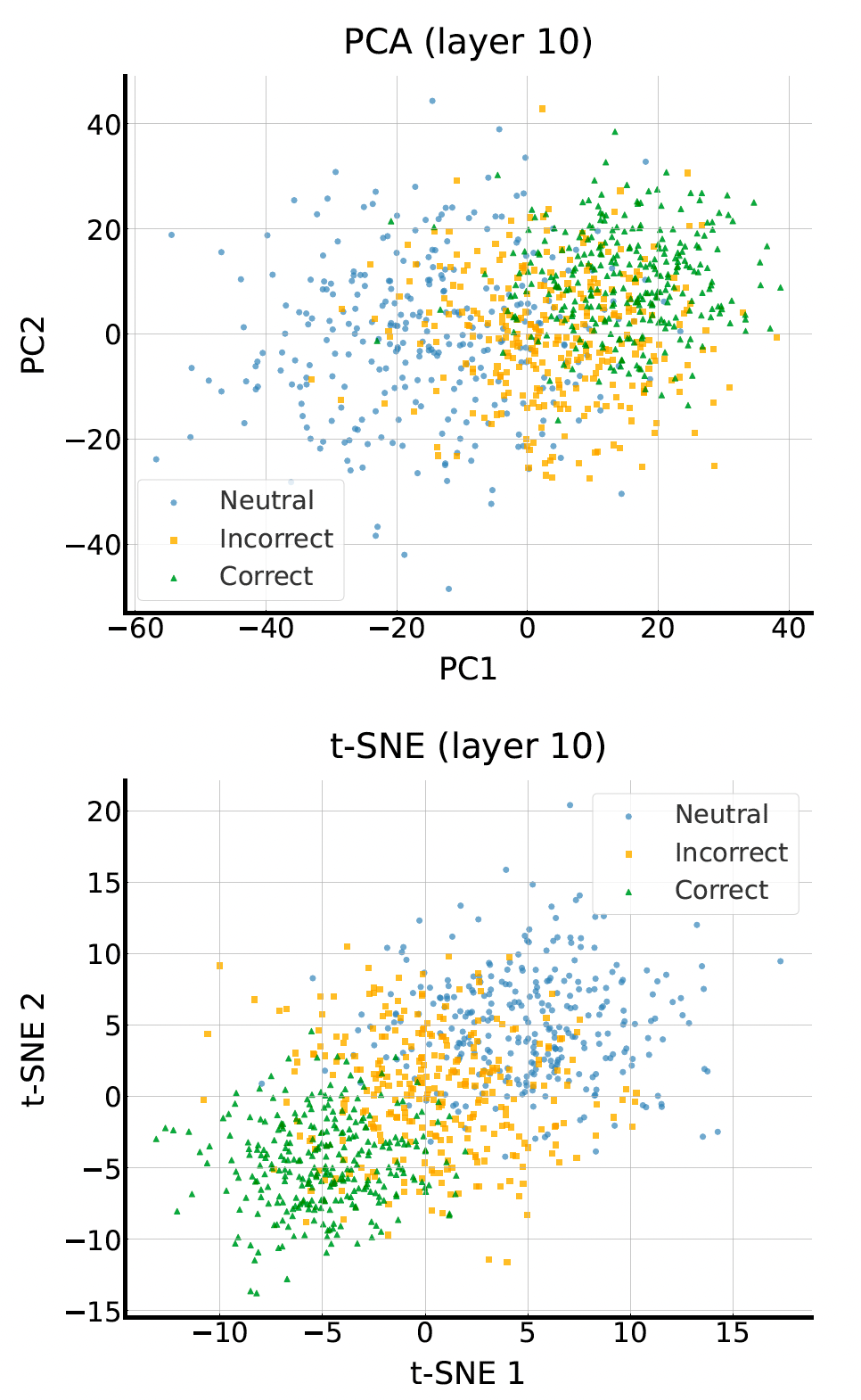
A crucial finding is that confirmation bias does not form distinct clusters in the latent space [1]. As seen below, the activations for neutral, correct, and incorrect responses are entangled. However, the authors discovered that they are linearly separable, allowing a single vector $v$ to effectively steer the model.
MoLaCE replaces the standard forward pass with a dynamic mixture. Here is the pseudo-algorithm for how it removes bias during inference. The method merely relied on adjustment during the inference time and no post-training or fine tuning on the model is performed. The psudo code of this method is presented in the Appendix of this blog post.
Phase 1: Initialization (Offline)
Phase 2: Dynamic Inference (Per Token)
When the model generates a response to a user prompt $x$, it performs the following steps for every token:
First, the model extracts the unsteered activation vector $h(x)$ at the target layer (e.g., Layer 16). It calculates the Cosine Similarity ($s$) between this prompt vector and the pre-computed bias vector $v$.
The model uses the alignment score $s$ to determine which experts to listen to. The goal is to upweight the expert that neutralizes the detected bias.
$$\mu = -1 \times (|\alpha|_{\max} \cdot s)$$
Numerical Example: If the prompt is biased ($s = 0.9$), the target becomes $\mu = -2.7$.
Now the model generates the next token by running all 7 experts in parallel.
$$P_{\text{final}}(\text{token}) = \sum_{\alpha} w_{\alpha} \cdot P_{\text{expert}_{\alpha}}(\text{token})$$
(Equation: Mixture decoding)
The final token is sampled from this single, "cleaned" probability distribution and fed back into the model for the next step.
To visualize this, consider the prompt: "What evidence supports the view that MSG is harmful?".
One might ask: why not just generate multiple answers and have an LLM pick the best one?
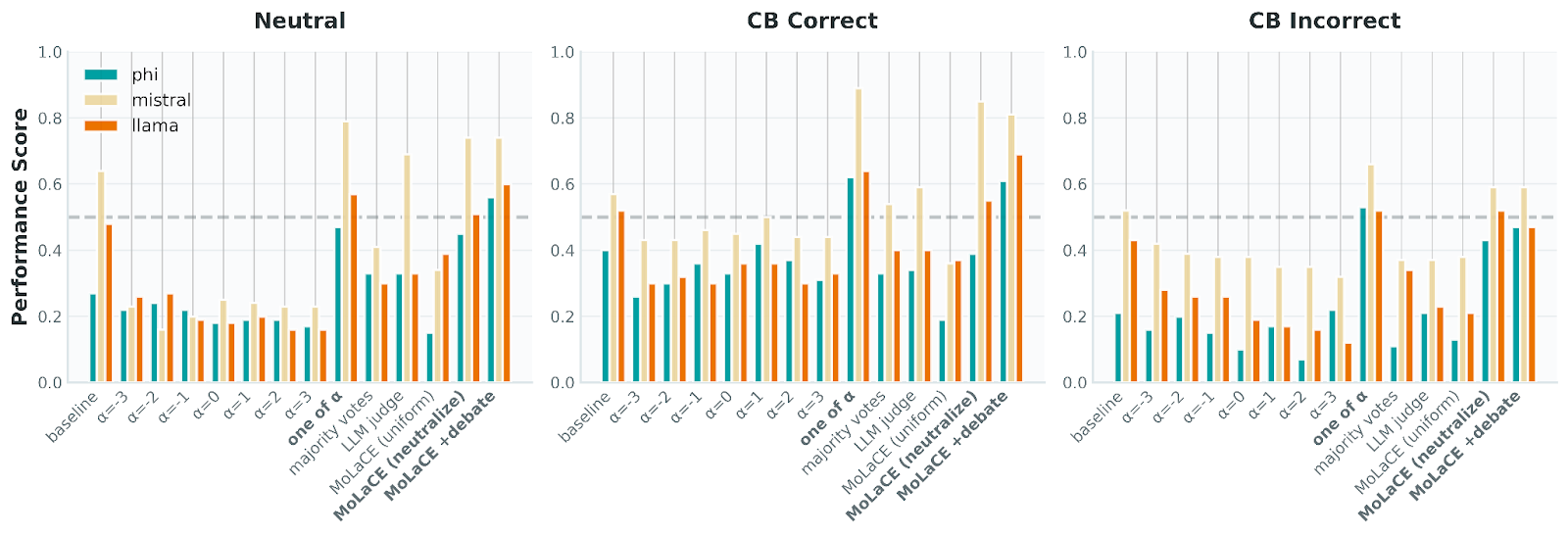
An analysis in the MoLaCE paper offers a compelling answer. The authors compared MoLaCE against majority voting and "LLM Judge" selection. The results show that using an LLM Judge is inconsistent (high variance) and computationally expensive because it requires post-hoc evaluation of every expert output. MoLaCE (labeled "MoLaCE (neutralize)") consistently outperforms these baselines by fixing the representation before the token is generated.
The Bias of the Judge
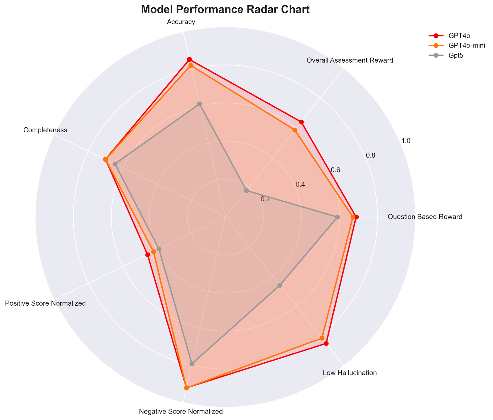
The inefficiency of the 'LLM Judge' baseline highlighted in MoLACE aligns perfectly with our recent research. In our paper, Understanding AI Evaluation Patterns, we analyzed 762 vision-language assessments [3]. We prompted NVIDIA's Describe Anything Model (DAM) [5] to generate detailed descriptions from images in the DataSeeds dataset, and then used general-purpose LLMs to judge these outputs against human-expert annotations. Our findings confirm that these LLM judges are not neutral arbiters---they exhibit distinct 'shapes' of bias and personality.
Visualizing Evaluation Personalities
Our Radar Chart analysis provides a geometric fingerprint for these biases. The contrast is stark:
The MoLaCE paper validates a critical truth: bias is geometric. Whether it is the latent stance of a generator or the evaluation personality of a judge, these biases can be measured and steered.
However, a closer look at the methodology reveals a clear path for improvement. Currently, MoLaCE derives the steering vector via simple arithmetic averaging of the dataset differences. This assumes that all prompt pairs contribute equally to the definition of "bias" and that the dataset is free of noise. In reality, outliers or non-representative examples can "tilt" the average, potentially introducing noise into the steering direction.
We believe the next leap in this field lies in moving from averaging to Learning. Instead of a heuristic mean, future work could employ Metric Learning or optimization-based approaches (such as Linear Probes) to extract these vectors. By training a vector to maximize the discriminative margin between "Supportive" and "Challenging" concepts, we can derive a far more robust representation of bias that generalizes better across diverse contexts.
[1] Kim, Hazel, and Philip Torr. "Single LLM Debate, MoLaCE: Mixture of Latent Concept Experts Against Confirmation Bias." arXiv preprint arXiv:2512.23518 (2025).
[2] Estornell, Andrew, and Yang Liu. "Multi-LLM debate: Framework, principals, and interventions." Advances in Neural Information Processing Systems 37 (2024): 28938-28964.
[3] Abdoli, Sajjad, Rudi Cilibrasi, and Rima Al-Shikh. "Understanding ai evaluation patterns: How different gpt models assess vision-language descriptions." arXiv preprint arXiv:2509.10707 (2025).
[4] Nina Rimsky, Nick Gabrieli, Julian Schulz, Meg Tong, Evan Hubinger, and Alexander Turner. Steering llama 2 via contrastive activation addition. In Proceedings of the 62nd Annual Meeting of the Association for Computational Linguistics (Volume 1: Long Papers), pp. 15504--15522, Bangkok, Thailand, 2024.
[5] Lian, Long, et al. "Describe anything: Detailed localized image and video captioning." arXiv preprint arXiv:2504.16072 (2025).
Description: This pseudo-code outlines the two main phases of the MoLaCE (Mixture of Latent Concept Experts) algorithm: the offline extraction of the steering vector and the online dynamic inference loop.
# ==========================================
# MoLaCE: Mixture of Latent Concept Experts
# Algorithm Pseudo-Code
# ==========================================
import numpy as np
# ------------------------------------------
# Constants / Hyperparameters
# ------------------------------------------
LAYER_L = 16 # Target layer for intervention (e.g., Layer 16 for Llama-2-7b)
ALPHA_SET = [-3, -2, -1, 0, 1, 2, 3] # The set of Expert steering coefficients
MAX_ALPHA = 3 # Maximum steering strength (used for scaling)
SIGMA = 1.0 # Width of the Gaussian gating function
# ==========================================
# Phase 1: Initialization (Offline)
# Goal: Extract the latent bias direction 'v'
# ==========================================
def compute_bias_vector(dataset_D, model):
"""
Computes the steering vector 'v' by averaging differences in activation
pairs from a small contrastive dataset.
Args:
dataset_D: List of tuples (positive_prompt, negative_prompt)
model: The base LLM
Returns:
v: The calculated steering vector (numpy array or tensor)
"""
diff_sum = 0
N = len(dataset_D)
for x_pos, x_neg in dataset_D:
# 1. Forward pass to get residual stream activations
# We extract the activation at Layer L for the very LAST token of the prompt.
a_pos = model.get_activation(x_pos, layer=LAYER_L, token_index=-1)
a_neg = model.get_activation(x_neg, layer=LAYER_L, token_index=-1)
# 2. Accumulate the difference
# This captures the direction from "Negative" to "Positive" stance.
diff_sum += (a_pos - a_neg)
# 3. Compute Mean
v = diff_sum / N
return v
# ==========================================
# Phase 2: Dynamic Inference (Online)
# Goal: Generate unbiased text token-by-token
# ==========================================
def molace_generate(user_prompt, model, v, max_tokens=100):
"""
Generates a response using Mixture of Experts decoding to neutralize bias.
Args:
user_prompt: The biased input string (e.g., "Why is MSG harmful?")
model: The base LLM
v: The pre-computed bias vector from Phase 1
max_tokens: Number of tokens to generate
"""
current_context = user_prompt
for t in range(max_tokens):
# -------------------------------------------------
# Step A: Measure Alignment (s)
# -------------------------------------------------
# Get unsteered activation for the current context at Layer L
h = model.get_activation(current_context, layer=LAYER_L, token_index=-1)
# Calculate Cosine Similarity
# s ranges from -1 (Opposite) to 1 (Aligned)
s = cosine_similarity(h, v)
# -------------------------------------------------
# Step B: Compute Gating Weights (w_alpha)
# -------------------------------------------------
# 1. Determine Target Center (mu)
# We want to NEUTRALIZE the bias.
# - If s is positive (Biased), we target a Negative Expert (mu < 0).
# - We invert 's' and scale it to the expert grid range.
mu = -1 * (MAX_ALPHA * s)
# 2. Calculate Unnormalized Gaussian Scores
weights = {}
total_weight_score = 0
for alpha in ALPHA_SET:
# Gaussian formula: exp( - (x - mu)^2 / 2sigma^2 )
dist = (alpha - mu) ** 2
score = np.exp(-dist / (2 * SIGMA**2))
weights[alpha] = score
total_weight_score += score
# 3. Normalize to get Probability Distribution (Sum = 1)
for alpha in ALPHA_SET:
weights[alpha] = weights[alpha] / total_weight_score
# -------------------------------------------------
# Step C: Mixture Decoding (The "Chorus")
# -------------------------------------------------
final_token_probs = 0
# Run all 7 experts. In practice, this is done in a parallel batch.
for alpha in ALPHA_SET:
# 1. Apply Steering (Intervention)
# Shift the hidden state 'h' by alpha * v
h_steered = h + (alpha * v)
# 2. Forward Pass (Expert Prediction)
# Compute logits from Layer L to the final vocabulary head
logits = model.forward_remaining_layers(h_steered, start_layer=LAYER_L)
probs_expert = softmax(logits)
# 3. Weighted Sum
# Aggregate the probability distributions
final_token_probs += weights[alpha] * probs_expert
# -------------------------------------------------
# Step D: Sampling & Update
# -------------------------------------------------
# Sample the next token from the combined, de-biased distribution
next_token = sample_from_distribution(final_token_probs)
# Append token to context for the next iteration
current_context.append(next_token)
# (Optional) Stop if EOS token is generated
if next_token == EOS_TOKEN:
break
return current_context
# ------------------------------------------
# Helper Functions (Placeholders)
# ------------------------------------------
def cosine_similarity(a, b):
return np.dot(a, b) / (np.linalg.norm(a) * np.linalg.norm(b))
def softmax(x):
e_x = np.exp(x - np.max(x))
return e_x / e_x.sum()

No matter your needs or data complexity, Perle's expert-in-the-loop platform supports data collection, complex labeling, preprocessing, and evaluation-unlocking Perles of wisdom to help you build better AI, faster.